CPD
Ouroboros Randomness Generation Sub-Protocol - The coin-flipping Problem
Cardano Problem Definition (CPD)
This document is a Cardano Problem Definition (CPD), from which the Cardano Problem Statement (CPS): Ouroboros Randomness Manipulation is derived.
While the CPS is being structured for formal submission with a focus on accessibility, and alignment with the CIP process, this CPD retains the full depth of technical material that shaped the problem understanding. It preserves detailed modeling, cost definitions, and adversarial analysis that could not be fully included in the CPS due to scope and formatting constraints.
The CPD thus complements the CPS by serving as its technical foundation and extended reference, providing the complete analytical context behind the identified problem.
Abstract
A well-designed consensus protocol is inherently modular, comprising multiple sub-protocols that collectively ensure security, efficiency, and decentralization. Among these, the Randomness Generation Sub-Protocol is pivotal in tackling the Coin-Flipping Problem—the challenge of generating fair, unbiased, and unpredictable randomness in a distributed environment.
This issue is especially critical in Ouroboros, where randomness underpins essential sub-protocols like leader election. A robust and tamper-resistant randomness mechanism is vital to maintaining the protocol’s security, fairness, and integrity.
This CPD delineates this challenge within the context of Ouroboros Praos, analyzing its approach and its vulnerability to grinding attacks, where adversaries attempt to manipulate leader election outcomes. The document offers:
- An analysis of attack vectors, their economic and computational prerequisites, and Cardano’s current resilience.
- A quantification of attack feasibility, highlighting escalation beyond a 20% stake threshold.
- Pivotal questions: Is manipulation occurring? What is Cardano’s vulnerability? How might threats be mitigated?
Rather than prescribing specific solutions, this CPD urges the Cardano community to take responsibility for addressing these risks, potentially through advancements in detection, stake distribution, or protocol design. It establishes a rigorous foundation for understanding these issues and solicits collaborative efforts to bolster Ouroboros’ resilience against evolving adversarial strategies.
Summary of Findings
This CPD undertakes a thorough examination of the Randomness Generation Sub-Protocol within the Ouroboros Praos, focusing on the Coin-Flipping Problem and its implications for the security of the Cardano blockchain. The principal findings are as follows:
- Randomness Mechanism: Ouroboros Praos utilizes VRFs for efficient randomness generation, yet this design exposes vulnerabilities to grinding attacks, wherein adversaries manipulate nonce values to influence leader election processes.
- Attack Feasibility: The likelihood and impact of successful attacks rise significantly when an adversary controls >20% of total stake (~4.36 billion ADA, March 2025), while lesser stakes render such efforts statistically improbable over extended periods.
- Economic Considerations: Acquiring substantial stake entails a significant financial commitment—on the order of billions of USD for a 20% share—further complicated by potential asset devaluation if an attack undermines network integrity.
- Computational Requirements: Scenario analysis across varying grinding depths () reveals a spectrum of feasibility:
- Minor attacks (e.g. manipulating blocks costs ~$56) are readily achievable.
- Significant manipulations (e.g. costs ~$3.1 billion) demand resources ranging from feasible to borderline infeasible, contingent upon adversary capabilities.
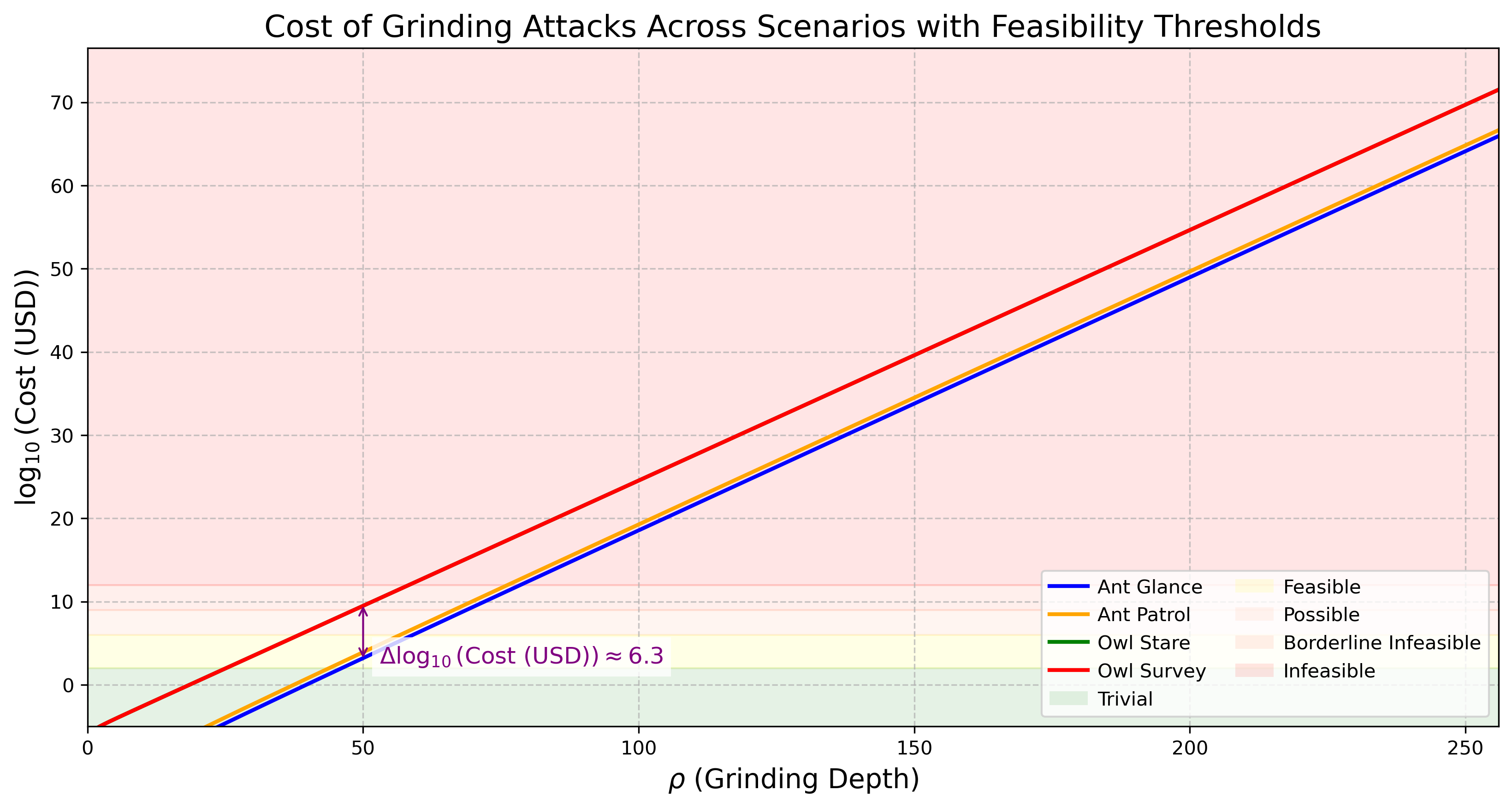
- The cost disparity between the most resource-intensive scenario (Owl Survey) and the least (Ant Glance) is substantial, with a consistent ratio of , indicating that the strongest attack here considered, the Owl Survey scenario, costs approximately times more than the base and weakest attack, Ant Glance, driven by the significant influence of the adversary's strategy evaluation, (simpled called the evaluation complexity), and their target window scope .
The table below delineates the values at which each scenario transitions across feasibility categories, illustrating the computational and economic thresholds:
| Feasibility Category | 🔵 Ant Glance | 🟠 Ant Patrol | 🟢 Owl Stare | 🔴 Owl Survey |
|---|---|---|---|---|
| 🟢 🌱 Trivial for Any Adversary | ||||
| 🟡 💰 Feasible with Standard Resources | ||||
| 🟠 🏭 Large-Scale Infrastructure Required | ||||
| 🔴 🚫 Borderline Infeasible | ||||
| 🔴 🚫 Infeasible |
✏️ Note: For a detailed explanation of these scenarios and their feasibility thresholds, refer to Section 3.5 - Scenarios within this CPD.
This document deliberately avoids advocating specific countermeasures, instead presenting these findings to highlight extant vulnerabilities and their associated costs. It is incumbent upon the Cardano community to assess and address these challenges, potentially through:
- Development of enhanced detection mechanisms,
- Improvement of stake pool diversity, or
- Introduction of protocol-level innovations.
Stakeholders are invited to engage with this CPD in its entirety to validate the analysis, deepen their comprehension, and assume ownership of subsequent solutions. Contributions are welcomed via the ongoing discourse at https://github.com/cardano-foundation/CIPs/pull/1009, aimed at collectively fortifying the Ouroboros protocol.
1. Preliminaries
This section introduces the pertinent parts of the Cardano proof-of-stake consensus protocol. We focus on the randomness generation and leader selection processes and omit irrelevant protocol details.
1.1 Fundamental Properties
A consensus protocol implements a robust transaction ledger if it maintains the ledger as a sequence of blocks, where each block is associated with a specific slot. Each slot can contain at most one ledger block, and this strict association ensures a well-defined and immutable ordering of transactions within the ledger.
The protocol must satisfy the two critical properties of Persistence and Liveness, which ensure that blocks and transactions are securely committed and cannot be easily manipulated by adversaries. These can be derived from fundamental chain properties which are used to explain how and why the leader election mechanism has been designed in this manner.
| Chain Property | Description |
|---|---|
| Common Prefix (CP) | Ensures consistency across honest parties by requiring that chains adopted by different honest nodes share a common prefix. |
| Existential Chain Quality (∃CQ) | Guarantees that at least one honestly-generated block appears in a portion of a sufficient length of the chain, ensuring honest contributions. |
| Chain Growth (CG) | Ensures that the blockchain extends at a minimum rate over time, preventing indefinite stalling by adversaries while maintaining progress based on the fraction of honest stakeholders producing blocks. |
1.1.1 Transaction Ledger Properties
1.1.1.1 Persistence with the security parameter k in N
Once a node of the system proclaims a certain transaction tx in the stable part of its ledger, all nodes, if queried, will either report tx in the same position of that ledger or report a stable ledger which is a prefix of that ledger. Here the notion of stability is a predicate that is parameterized by a security parameter k. Specifically, a transaction is declared stable if and only if it is in a block that is more than k blocks deep in the ledger.
1.1.1.2 Liveness with the transaction confirmation time parameter u in N
If all honest nodes in the system attempt to include a certain transaction then, after the passing of time corresponding to u slots (called the transaction confirmation time), all nodes, if queried and responding honestly, will report the transaction as stable.
1.1.2 Chain properties
Persistence and liveness can be derived from basic chain properties, provided that the protocol structures the ledger as a blockchain—a sequential data structure. The following key chain properties ensure that the blockchain behaves securely and efficiently:
1.1.2.1 Common Prefix (CP): With the security parameter k in N
Consider 2 chains and adopted by 2 honest parties at the onset of slots and , respectively, where . The chains must satisfy the condition:
Where:
- represents the chain obtained by removing the last blocks from .
- denotes the prefix relation.
This ensures that the shorter chain is a prefix of the longer one, ensuring consistency across honest parties.
1.1.2.2 Existential Chain Quality (∃CQ): With parameter s in N (Minimum Honest Block Inclusion Interval)
Consider a chain adopted by an honest party at the onset of a slot. For any portion of spanning prior slots, there must be at least one honestly-generated block within this portion. This ensures that the chain includes contributions from honest participants. In practical terms, defines the length of a "safety window" where honest contributions are guaranteed.
1.1.2.3 Chain Growth (CG): With parameters tau in (0, 1] (speed coefficient) and s in N (Minimum Honest Block Inclusion Interval)
The Chain Growth (CG) property is a more general concept that combines both the speed of block production and the frequency of honest contributions. It uses two parameters: , the speed coefficient, which governs how fast the chain grows, and , the Minimum Honest Block Inclusion Interval, which ensures that honest blocks are consistently produced within a given interval of slots.
Consider a chain held by an honest party at the onset of a slot. For any portion of spanning contiguous prior slots . The number of blocks in this portion must be at least . The parameter determines the fraction of slots in which blocks are produced. For example, if and , there should be at least 5 blocks produced within that span.
For example, if and , then at least honest blocks must be produced over the span of those 10 slots.
1.2 The Coin-Flipping Problem
The Coin-Flipping Problem is a fundamental challenge in distributed systems that require a fair, unbiased, and unpredictable source of randomness—without allowing any single participant to manipulate the outcome.
1.2.1 Defining the Problem
Consider a scenario where multiple untrusted parties must flip a coin and use the outcome, the concatenation of heads or tails, to reach a decision. The challenge is ensuring that:
- 🎲 The outcome remains random and unpredictable.
- 🔒 No participant can bias or influence the result in their favor.
- ⚖️ The process is fair and secure, even in the presence of dishonest or colluding actors.
In blockchain consensus protocols, randomness is crucial for leader election, committee selection, and cryptographic lotteries. If an adversary can bias the randomness, they can increase their influence over block production, delay settlements, or disrupt network security.
1.2.2 Strategies for Randomness Generation
Various cryptographic techniques exist to address the coin-flipping problem in decentralized settings. These methods differ in security, efficiency, and resistance to adversarial manipulation.
| Approach | Pros | Cons |
|---|---|---|
| PVSS-Based Beacons (Ouroboros Classic, RandHound, Scrape, HydRand) | ✔ Strong randomness guarantees — output is indistinguishable from uniform. ✔ Resistant to last-mover bias — commitments prevent selective reveals. | ❌ High communication complexity — requires O(n²) messages. ❌ Vulnerable to adaptive adversaries — who may corrupt committee members. |
| Threshold Signature-Based Beacons (DFINITY) | ✔ Fast and non-interactive — requires only one round of communication. ✔ Resistant to last-mover bias — output is deterministic. | ❌ Group setup complexity — requires distributed key generation (DKG). ❌ No random number output in case of threshold signature generation failure. |
| Byzantine Agreement-Based Beacons (Algorand) | ✔ Finality guarantees — randomness is confirmed before the next epoch. ✔ Less entropy loss than Praos. | ❌ Requires multi-round communication — higher latency. ❌ Not designed for eventual consensus — better suited for BA-based protocols. |
| "VRF"-Based Beacons (Ethereum’s RANDAO Post-Merge, Ouroboros Praos, Genesis, Snow White) | ✔ Simple and efficient — low computational overhead. ✔ Fully decentralized — any participant can contribute randomness. | ❌ Vulnerable to last-revealer bias — the last participant can manipulate the final output. |
1.2.3 The Historical Evolution of Ouroboros Randomness Generation
The Ouroboros family of protocols has evolved over time to optimize randomness generation while balancing security, efficiency, and decentralization. Initially, Ouroboros Classic used a secure multi-party computation (MPC) protocol with Publicly Verifiable Secret Sharing (PVSS) to ensure unbiased randomness. While providing strong security guarantees, PVSS required quadratic message exchanges between committee members, introducing significant communication overhead. This scalability bottleneck limited participation and hindered the decentralization of Cardano's consensus process.
Recognizing these limitations, Ouroboros Praos moved to a VRF-based randomness generation mechanism where each individual randomness contribution is generated with Verifiable Random Functions (VRFs). Here, each block includes a VRF value, that is a veriable random value that gas been deterministically computed from a fixed message. The random nonce for an epoch is then derived from the concatenation and hashing of all these values from a specific section of the previous epoch’s chain. This significantly reduces the communication complexity, which now becomes linear in the number of block producers, making randomness generation scalable and practical while maintaining adequate security properties.
However, this efficiency gain comes at a cost: the random nonce is now biasable as this protocol change introduces a limited avenue for randomness manipulation. Adversaries can attempt grinding attacks, evaluating multiple potential nonces and selectively influencing randomness outcomes. While constrained, this trade-off necessitates further countermeasures to limit adversarial influence while maintaining protocol scalability.
📌📌 More Details on VRFs – Expand to view the content.
Verifiable Random Functions (VRFs) are cryptographic primitives that produce a pseudorandom output along with a proof that the output was correctly generated from a given input and secret key.
BLS Signatures (Boneh–Lynn–Shacham) can be used as Verifiable Random Functions (VRFs) because they satisfy the core properties — Determinism, Pseudorandom and efficiently Verifiable - required of a VRF.
A BLS signature is indistinguishable from random without knowledge of the secret key, their signature is efficient and the signature generation is determistic and secure under standard cryptographic assumptions.
1.2.4 Comparing Ouroboros Randomness Generation with Ethereum
Ethereum RANDAO protocol was first based on a commit and reveal approach where each block producer would commit to random values in a first period, i.e. publish the hash of a locally generated random value during block proposal, before revealing them afterwards. As the latter period finished, all revealed values were combined, more specifically XORed, together to finally get the random nonce.
Ethereum's Post-Merge RANDAO protocol remains mostly the same, but instead of using a commit-reveal approach, each contributor generate randomness deterministically by using VRFs, making these values verifiable. These values are finally, as before, sequentially aggregated using XOR, forming the final randomness output used in validator shuffling and protocol randomness. This version of the protocol is very similar to Ouroboros Praos' where hashing is used instead of XOR to combine contributors' randomness together, and does not rely on commitees.
While decentralized and computationally lightweight, RANDAO still suffers from last-revealer bias, where the final proposers in an epoch can withhold their reveals to manipulate randomness. As such, Ethereum has spent some time studying Verifiable Delayed Functions (VDFs) to prevent the last revealer attack by relying on its sequentiality property. Subsequently, Ethereum decided against integrating Verifiable Delay Functions due to feasibility concerns, including the difficulty of practical deployment and the risk of centralization stemming from specialized hardware dependencies. They instead opted for a frequent reseeding mechanism to strengthen the commitee selection in order to mitigate biases which, unfortunately does not fully eliminate last-revealer manipulation concerns.
📌📌 More Details on VDFs – Expand to view the content.
VDFs are designed to provide unpredictable, verifiable randomness by requiring a sequential computation delay before revealing the output.
This makes them resistant to grinding attacks since adversaries cannot efficiently evaluate multiple outcomes. However, they introduce significant computational costs, require specialized hardware for efficient verification, and demand additional synchronization mechanisms.
1.2.5 Conclusion: The reasons behind Ouroboros Praos
Despite some security trade-offs, non-interactively combining VRFs was selected for Ouroboros Praos due to its balance between efficiency, scalability, and security. Unlike PVSS, we do not require a multi-party commit-reveal process or have quadratic communication overhead.
However, ongoing research continues to explore potential enhancements to mitigate grinding risks, including hybrid randomness beacons that combine VRFs with cryptographic delay mechanisms.
1.3 Leader Election in Praos
1.3.1 Oblivious Leader Selection
As Explained into DGKR18 - Ouroboros Praos_ An adaptively-secure, semi-synchronous proof-of-stake blockchain, Praos protocol presents the following basic characteristics :
-
Slot Leader Privacy: Only the selected leader knows they have been chosen as slot leader until they reveal themselves, often by publishing a proof. This minimizes the risk of targeted attacks against the leader since other network participants are unaware of the leader's identity during the selection process.
-
Verifiable Randomness: The selection process uses verifiable randomness functions (VRFs) to ensure that the leader is chosen fairly, unpredictably, and verifiably. The VRF output acts as a cryptographic proof that the selection was both random and valid, meaning others can verify it without needing to know the leader in advance.
-
Low Communication Overhead: Since the identity of the leader is hidden until the proof is revealed, Oblivious Leader Selection can reduce communication overhead and minimize the chance of network-level attacks, such as Distributed Denial of Service (DDoS) attacks, aimed at preventing the leader from performing their role.
Based on their local view, a party is capable of deciding, in a publicly verifiable way, whether they are permitted to produce the next block, they are called a slot leader. Assuming the block is valid, other parties update their local views by adopting the block, and proceed in this way continuously. At any moment, the probability of being permitted to issue a block is proportional to the relative stake a player has in the system, as reported by the blockchain itself :
- potentially, multiple slot leaders may be elected for a particular slot (forming a slot leader set);
- frequently, slots will have no leaders assigned to them; This is defined by the Active Slot Coefficient f
- a priori, only a slot leader is aware that it is indeed a leader for a given slot; this assignment is unknown to all the other stakeholders—including other slot leaders of the same slot—until the other stakeholders receive a valid block from this slot leader.
1.3.2 Application of Verifiable Random Function (VRF)
The VRF is used to generate randomness locally in the protocol, making the leader election process unpredictable. It ensures that:
- A participant is privately and verifiably selected to create a block for a given slot.
- The VRF output is both secret (only known to the selected leader) and verifiable (publicly checkable).
To determine whether a participant is the slot leader of in epoch , they first generate a VRF output and proof using their secret VRF key out of the slot number and current epoch random nonce . They then compare this value with a threshold that is computed from the participant's relative stake at the beginning of the epoch. If the VRF output is smaller than the threshold, they become the slot leader of . In that case, when publishing a block for this slot, they include in the block header , the comprising the VRF proof.
| Features | Mathematical Formula | Description |
|---|---|---|
| Slot Leader Proof | This function computes the leader eligibility proof using the VRF, based on the slot number and randomness nonce. | |
| Slot Leader Threshold | This function calculates the threshold for a participant's eligibility to be selected as a slot leader during . | |
| Eligibility Check | The leader proof is compared against a threshold to determine if the participant is eligible to create a block. | |
| Verification | Other nodes verify the correctness of the leader proof by recomputing it using the public VRF key and slot-specific input. |
| Where | |
|---|---|
| The current slot number. | |
| Eta, The randomness nonce used in , computed within the previous . | |
| The node's secret (private) key. | |
| The node's public key. | |
| Generate a Certification with input | |
| Verify a Certification with input | |
| The concatenation of and , followed by a BLAKE2b-256 hash computation. | |
| The stake owned by the participant used in , computed within the previous | |
| The total stake in the system used in , computed within the previous | |
| The active slot coefficient (referred as ), representing the fraction of slots that will have a leader and eventually a block produced. |
📌📌 Relevant Implementation Code Snippets for This Section – Expand to view the content.
-- | The body of the header is the part which gets hashed to form the hash
-- chain.
data HeaderBody crypto = HeaderBody
  { -- | block number
    hbBlockNo  :: !BlockNo,
    -- | block slot
    hbSlotNo   :: !SlotNo,
    -- | Hash of the previous block header
    hbPrev     :: !(PrevHash crypto),
    -- | verification key of block issuer
    hbVk       :: !(VKey 'BlockIssuer crypto),
    -- | VRF verification key for block issuer
    hbVrfVk    :: !(VerKeyVRF crypto),
    -- | Certified VRF value
    hbVrfRes   :: !(CertifiedVRF crypto InputVRF),
    -- | Size of the block body
    hbBodySize :: !Word32,
    -- | Hash of block body
    hbBodyHash :: !(Hash crypto EraIndependentBlockBody),
    -- | operational certificate
    hbOCert    :: !(OCert crypto),
    -- | protocol version
    hbProtVer  :: !ProtVer
  }
  deriving (Generic)

-- | Input to the verifiable random function. Consists of the hash of the slot
-- and the epoch nonce.
newtype InputVRF = InputVRF {unInputVRF :: Hash Blake2b_256 InputVRF}
  deriving (Eq, Ord, Show, Generic)
  deriving newtype (NoThunks, ToCBOR)

-- | Construct a unified VRF value
mkInputVRF ::
  SlotNo ->
  -- | Epoch nonce
  Nonce ->
  InputVRF
mkInputVRF (SlotNo slot) eNonce =
  InputVRF
    . Hash.castHash
    . Hash.hashWith id
    . runByteBuilder (8 + 32)
    $ BS.word64BE slot
      <> ( case eNonce of
             NeutralNonce -> mempty
             Nonce h      -> BS.byteStringCopy (Hash.hashToBytes h)
         )

-- | Assert that a natural is bounded by a certain value. Throws an error when
-- this is not the case.
assertBoundedNatural ::
  -- | Maximum bound
  Natural ->
  -- | Value
  Natural ->
  BoundedNatural
assertBoundedNatural maxVal val =
  if val <= maxVal
    then UnsafeBoundedNatural maxVal val
    else error $ show val <> " is greater than max value " <> show maxVal

-- | The output bytes of the VRF interpreted as a big endian natural number.
--
-- The range of this number is determined by the size of the VRF output bytes.
-- It is thus in the range @0 ..  2 ^ (8 * sizeOutputVRF proxy) - 1@.
--
getOutputVRFNatural :: OutputVRF v -> Natural
getOutputVRFNatural = bytesToNatural . getOutputVRFBytes

-- This is fast enough to use in production.
bytesToNatural :: ByteString -> Natural
bytesToNatural = GHC.naturalFromInteger . bytesToInteger

bytesToInteger :: ByteString -> Integer
bytesToInteger (BS.PS fp (GHC.I# off#) (GHC.I# len#)) =
  -- This should be safe since we're simply reading from ByteString (which is
  -- immutable) and GMP allocates a new memory for the Integer, i.e., there is
  -- no mutation involved.
  unsafeDupablePerformIO $
    withForeignPtr fp $ \(GHC.Ptr addr#) ->
      let addrOff# = addr# `GHC.plusAddr#` off#
       in -- The last parmaeter (`1#`) tells the import function to use big
          -- endian encoding.
          importIntegerFromAddr addrOff# (GHC.int2Word# len#) 1#
  where
    importIntegerFromAddr :: Addr# -> Word# -> Int# -> IO Integer
#if __GLASGOW_HASKELL__ >= 900
-- Use the GHC version here because this is compiler dependent, and only indirectly lib dependent.
    importIntegerFromAddr addr sz = integerFromAddr sz addr
#else
    importIntegerFromAddr = GMP.importIntegerFromAddr
#endif


-- | Check that the certified VRF output, when used as a natural, is valid for
-- being slot leader.
checkLeaderValue ::
  forall v.
  VRF.VRFAlgorithm v =>
  VRF.OutputVRF v ->
  Rational ->
  ActiveSlotCoeff ->
  Bool
checkLeaderValue certVRF σ f =
  checkLeaderNatValue (assertBoundedNatural certNatMax (VRF.getOutputVRFNatural certVRF)) σ f
  where
    certNatMax :: Natural
    certNatMax = (2 :: Natural) ^ (8 * VRF.sizeOutputVRF certVRF)

-- | Check that the certified input natural is valid for being slot leader. This
-- means we check that
--
-- p < 1 - (1 - f)^σ
--
-- where p = certNat / certNatMax.
--
-- The calculation is done using the following optimization:
--
-- let q = 1 - p and c = ln(1 - f)
--
-- then           p < 1 - (1 - f)^σ
-- <=>  1 / (1 - p) < exp(-σ * c)
-- <=>  1 / q       < exp(-σ * c)
--
-- This can be efficiently be computed by `taylorExpCmp` which returns `ABOVE`
-- in case the reference value `1 / (1 - p)` is above the exponential function
-- at `-σ * c`, `BELOW` if it is below or `MaxReached` if it couldn't
-- conclusively compute this within the given iteration bounds.
--
-- Note that  1       1               1                         certNatMax
--           --- =  ----- = ---------------------------- = ----------------------
--            q     1 - p    1 - (certNat / certNatMax)    (certNatMax - certNat)
checkLeaderNatValue ::
  -- | Certified nat value
  BoundedNatural ->
  -- | Stake proportion
  Rational ->
  ActiveSlotCoeff ->
  Bool
checkLeaderNatValue bn σ f =
  if activeSlotVal f == maxBound
    then -- If the active slot coefficient is equal to one,
    -- then nearly every stake pool can produce a block every slot.
    -- In this degenerate case, where ln (1-f) is not defined,
    -- we let the VRF leader check always succeed.
    -- This is a testing convenience, the active slot coefficient should not
    -- bet set above one half otherwise.
      True
    else case taylorExpCmp 3 recip_q x of
      ABOVE _ _ -> False
      BELOW _ _ -> True
      MaxReached _ -> False
  where
    c, recip_q, x :: FixedPoint
    c = activeSlotLog f
    recip_q = fromRational (toInteger certNatMax % toInteger (certNatMax - certNat))
    x = -fromRational σ * c
    certNatMax = bvMaxValue bn
    certNat = bvValue bn

  -- | Evolving nonce type.
data Nonce
  = Nonce !(Hash Blake2b_256 Nonce)
  | -- | Identity element
    NeutralNonce
  deriving (Eq, Generic, Ord, Show, NFData)

-- | Evolve the nonce
(⭒) :: Nonce -> Nonce -> Nonce
Nonce a ⭒ Nonce b =
  Nonce . castHash $
    hashWith id (hashToBytes a <> hashToBytes b)
x ⭒ NeutralNonce = x
NeutralNonce ⭒ x = x

-- | Hash the given value, using a serialisation function to turn it into bytes.
--
hashWith :: forall h a. HashAlgorithm h => (a -> ByteString) -> a -> Hash h a
hashWith serialise =
    UnsafeHashRep
  . packPinnedBytes
  . digest (Proxy :: Proxy h)
  . serialise

instance HashAlgorithm Blake2b_224 where
  type SizeHash Blake2b_224 = 28
  hashAlgorithmName _ = "blake2b_224"
  digest _ = blake2b_libsodium 28

blake2b_libsodium :: Int -> B.ByteString -> B.ByteString
blake2b_libsodium size input =
  BI.unsafeCreate size $ \outptr ->
    B.useAsCStringLen input $ \(inptr, inputlen) -> do
      res <- c_crypto_generichash_blake2b (castPtr outptr) (fromIntegral size) (castPtr inptr) (fromIntegral inputlen) nullPtr 0 -- we used unkeyed hash
      unless (res == 0) $ do
        errno <- getErrno
        ioException $ errnoToIOError "digest @Blake2b: crypto_generichash_blake2b" errno Nothing Nothing
1.3.3 Epoch Structure
In Praos and Genesis, an epoch consists of 3 logical phases to compute these 2 key variables—active stake distribution and randomness beacon—by going through the following phases:
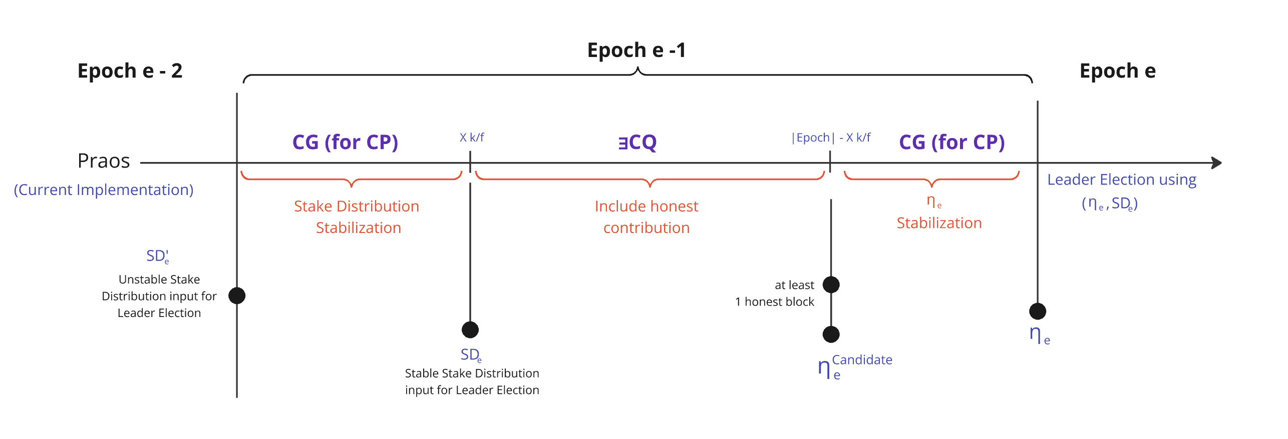
The sequential flow of these 3 phases is deliberately structured by designed :
| Id | Phase | Key Property | Description |
|---|---|---|---|
| 1. | Stabilization | Chain Growth (CG for CP) | This phase must be long enough to satisfy the Chain Growth (CG) property, ensuring that each honest party's chain grows by at least blocks. This guarantees that all honest parties agree on the stake distribution from the previous epoch. |
| 2. | Honest Randomness in | Existential Chain Quality (∃CQ) | After the Active Stake Distribution being stabilized to prevent adversaries from adjusting their stake in their favor, this phase must be sufficiently long to satisfy the Existential Chain Quality (∃CQ) property, which is parameterized by , ensuring that at least one honestly-generated block is included within any span of slots. The presence of such a block guarantees that honest contributions to the randomness used in the leader election process are incorporated. This phase directly improves the quality of the randomness by ensuring that adversarial attempts to manipulate the randomness beacon are mitigated. The honest block serves as a critical input, strengthening the unpredictability and fairness of the leader election mechanism. |
| 3. | Stabilization | Chain Growth (CG for CP) | This phase must again be long enough to satisfy the Chain Growth (CG) property, ensuring that each honest party's chain grows by at least blocks, allowing all honest parties to agree on the randomness contributions from the second phase. |
1.3.4 Epoch & Phases Length
While there is no theoretical upper bound on the epoch size—since it is defined by social and practical considerations (e.g., slots, 5 days)—the epoch does have a defined lower bound. Phases 1 and 3 have fixed sizes of and , respectively. The size of Phase 2, "Honest Randomness in ," is adjustable with a minimum size of .
The structure of an epoch is often described by the ratio 3:3:4:
- Phase 1 occupies 3 parts of the total epoch.
- Phase 2 also occupies 3 parts of the epoch (adjusted slightly to ensure the total reaches 10 parts in total.).
- Phase 3 takes up the remaining 4 parts of the epoch.
Note that the third phase is only longer than the first one to complete the epoch duration. Consequently, we can assume that the CG property is already reached at the ninth part of an epoch.
1.3.5 The Randomness Generation Sub-Protocol
To select the slots leaders, which stake pool is eligible to produce and propose a slot's block, we need to rely on random numbers. As economic reward and transaction inclusion depends on these numbers, the generation of these number is of critical importance to the protocol and its security. We show in this section how these random numbers, or random nonces are defined.
The eta-evolving Stream Definition
Contrary to Section 1.2.3, where we first defined the random nonce as the hash of all VRF outputs, we adopt an iterative approach for the randomness generation in practice. More particularly, the random nonces are defined iteratively from a genesis value, as the hash of the previous epoch's nonce and the VRF outputs published between the Phase 2 of consecutive epochs. We thus talk about evolving nonces as their value can be updated with the VRF output comprised in each block.
| where | |
|---|---|
| The evolving nonce is initialized using the extra Entropy field defined in the protocol parameters. | |
| The VRF output generated by the Leader and included in the block header | |
| The concatenation of and , followed by a BLAKE2b-256 hash computation. |
The candidates
-
As multiple competing forks can exist at any given time, we also encounter multiple nonce candidates, denoted as . More precisely, the nonce candidate of a specific fork for epoch is derived from the previous epoch’s nonce , the Verifiable Random Function (VRF) outputs from the candidate chain starting from epoch , and the VRF outputs of the fork itself up to the end of Phase 2 of epoch .
-
These components together form a candidate nonce for epoch , corresponding to the last derived evolving nonce at the conclusion of Phase 2 of epoch :
The Generations
- This is the final nonce used to determine participant eligibility during epoch .
- The value of is derived from the contained within the fork that is ultimately selected as the canonical chain at the conclusion of .
- It originates from concatenated with of the last block of the previous epoch followed by a BLAKE2b-256 hash computation , which becomes stabilized at the conclusion of and transitions into .
As one of these fork will become the canonical main chain, so will the candidate nonce. Hence, the epoch nonce is the candidate nonce of the longest chain at Phase 2, which is determined once the chain stabilises.
For a detailed formalization of the consensus mechanisms discussed herein, refer to the Consensus Specifications in the Cardano Formal Specifications repository maintained by IntersectMBO.
📌📌 Divergence with academic papers – Expand to view the content .
In the Ouroboros Praos paper, an epoch's random nonce is computed as the hash of the first blocks' VRF outputs, combined with some auxiliary information. This design ensures that individual random contributions are published on-chain, publicly verifiable, and that the final randomness computation remains efficient.
However, in practice, slight modifications were introduced to distribute the nonce generation cost across the network. This was achieved by iterative hashing, which not only balances the computational load but also ensures uniform block generation behavior regardless of a block's position within the epoch.
The nonce aggregates randomness from the entire epoch, rather than a limited subset as described in the academic version of the paper. When generating the nonce for epoch , we incorporate:
- VRF outputs from Phase 3 of epoch
- VRF outputs from Phases 1 and 2 of epoch
- The previous epoch's nonce
This leads to the following iterative hashing process:
This approach contrasts with the simpler method from the paper, where only the VRF outputs of Phase 1 and 2 of epoch are hashed together with :
📌📌 Relevant Implementation Code Snippets for This Section – Expand to view the content.
  -- | Evolving nonce type.
data Nonce
  = Nonce !(Hash Blake2b_256 Nonce)
  | -- | Identity element
    NeutralNonce
  deriving (Eq, Generic, Ord, Show, NFData)

-- | Evolve the nonce
(⭒) :: Nonce -> Nonce -> Nonce
Nonce a ⭒ Nonce b =
  Nonce . castHash $
    hashWith id (hashToBytes a <> hashToBytes b)
x ⭒ NeutralNonce = x
NeutralNonce ⭒ x = x

-- | Hash the given value, using a serialisation function to turn it into bytes.
--
hashWith :: forall h a. HashAlgorithm h => (a -> ByteString) -> a -> Hash h a
hashWith serialise =
    UnsafeHashRep
  . packPinnedBytes
  . digest (Proxy :: Proxy h)
  . serialise

instance HashAlgorithm Blake2b_224 where
  type SizeHash Blake2b_224 = 28
  hashAlgorithmName _ = "blake2b_224"
  digest _ = blake2b_libsodium 28

blake2b_libsodium :: Int -> B.ByteString -> B.ByteString
blake2b_libsodium size input =
  BI.unsafeCreate size $ \outptr ->
    B.useAsCStringLen input $ \(inptr, inputlen) -> do
      res <- c_crypto_generichash_blake2b (castPtr outptr) (fromIntegral size) (castPtr inptr) (fromIntegral inputlen) nullPtr 0 -- we used unkeyed hash
      unless (res == 0) $ do
        errno <- getErrno
        ioException $ errnoToIOError "digest @Blake2b: crypto_generichash_blake2b" errno Nothing Nothing
1.4 Forks, Rollbacks, Finality, and Settlement Times
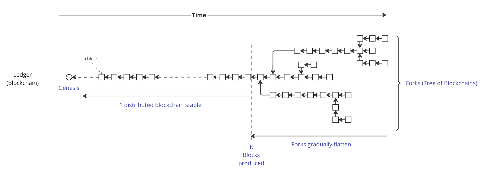
With Ouroboros Praos, as with Nakamoto consensus in general, transaction finality is probabilistic rather than immediate. This means a transaction isn't guaranteed to be permanently stored in the ledger when it's first included in a block. Instead, each additional block added on top strengthens its permanence, gradually decreasing the likelihood of a rollback.
Ouroboros Praos guarantees that after blocks have been produced, the likelihood of a rollback diminishes to the point where those blocks can be regarded as secure and permanent within the ledger. However, before these blocks are finalized, multiple versions of the blockchain — commonly referred to as "forks" — may coexist across the network. Each fork represents a potential ledger state until finality is ultimately achieved.
The consensus layer operates with a structure that resembles a branching "tree" of blockchains before finality stabilizes:
Why Do Blockchain Forks Occur?
Blockchain forks can happen for several reasons:
- Multiple slot leaders can be elected for a single slot, potentially resulting in the production of multiple blocks within that slot.
- Block propagation across the network takes time, causing nodes to have differing views of the current chain.
- Nodes can dynamically join or leave the network, which is a fundamental challenge in decentralized systems, affecting synchronization and consensus stability.
- An adversarial node is not obligated to agree with the most recent block (or series of blocks); it can instead choose to append its block to an earlier block in the chain.
Short Forks vs. Long Forks
Short forks, typically just a few blocks long, occur frequently and are usually non-problematic. The rolled-back blocks are often nearly identical, containing the same transactions, though they might be distributed differently among the blocks or have minor differences.
However, longer forks can have harmful consequences. For example, if an end-user (the recipient of funds) makes a decision—such as accepting payment and delivering goods to another user (the sender of the transaction)—based on a transaction that is later rolled back and does not reappear because it was invalid (e.g., due to double-spending a UTxO), it creates a risk of fraud.
2. The Grinding Attack Algorithm
This section describes the grinding attack, detailing its objectives, mechanics, and the adversary’s strategy to maximize its effectiveness.
2.1 Randomness Manipulation
We describe here the grinding attack Cardano's randomness generation protocol suffers from, from passively waiting for its chance or actively maximizing its attack surface, to choosing the best attack vector - stake distribution - to achieve its goal, be it maximizing rewards to controlling target blocks.
2.1.1 Exposure
In its current version, Praos has a vulnerability where an adversary can manipulate the nonce , the random value used for selecting block producers. This allows the adversary to incrementally and iteratively undermine the uniform distribution of slot leaders, threatening the fairness and unpredictability of the leader selection process.
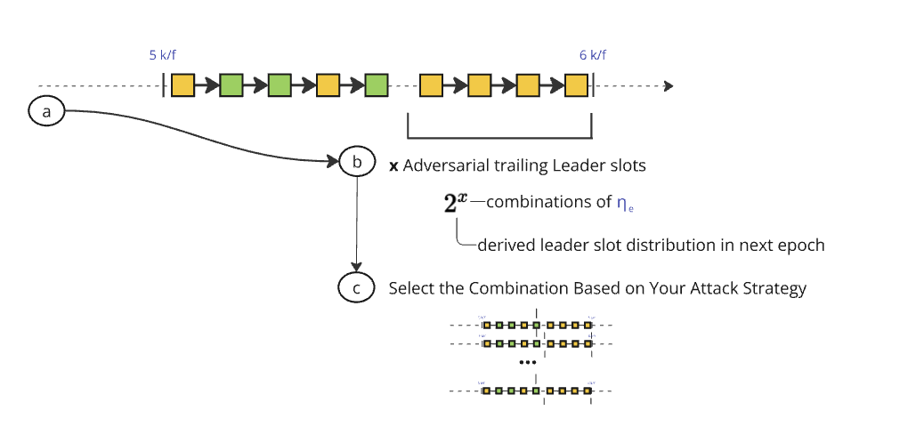
At the conclusion of Phase 2, when the nonce is determined, the distribution of slot leaders for the next epoch becomes deterministic in a private manner. This means that, at this point, the adversary gains precise knowledge of the slots in which they will be elected but lacks detailed knowledge of the slot distribution for honest participants.
For example, if the adversary acts as the slot leader immediately before this phase transition, they can choose whether to produce a block or not. This decision grants them the ability to compute and compare two valid nonces - one with one fewer VRF update than the other -, evaluate different slot leader distributions for the upcoming epoch and potentially maximize their future gains at the cost of lesser rewards at this epoch. The more blocks the adversary controls before Phase 2's end, the more nonces they may grind and choose from, and the more critical the attack becomes. In essence, the adversary gains access to up to possible combinations of slot leader distributions, where denotes the number of controlled leader slots at this particular stage of the protocol.
This marks the beginning of a grinding attack, where the adversary's initial goal is to maximize the number of adversarial blocks at this critical juncture, either passively by waiting, or actively by reaching a snowball effect. By doing so, they expand the range of potential slot leader distributions they can choose from, significantly enhancing their influence over the protocol. We use the term "exposure" here because the adversary is first setting the stage for its attack.
2.1.2 Slot Leader Distribution Selection
This is the pivotal moment where the adversary's prior efforts pay off. They are now in a position with x blocks at the critical juncture. At this stage, the adversary can generate up to possible nonces, compute the next epoch's slot leader distribution for each of them, and strategically select the nonce and distribution that best aligns with their goal. This positioning enables them to deploy the attack effectively in the subsequent epoch.
As the adversary accumulates blocks, the attack's bottleneck swiftly shifts from waiting for enough blocks at the critical juncture to the computational power needed to compute enough nonces to achieve their goal.
Accumulating a significant number of leader slots at this position necessitates, except when owning a significant portion of the total stake, an underlying intent to exploit or destabilize the protocol. Achieving such a level of control requires significant coordination, making it highly unlikely to occur without deliberate adversarial motives. Once an attacker reaches this threshold, their objectives extend beyond a single exploit and diversify into various strategic threats.
2.1.3 Potential Outcomes of Grinding Attacks
Below is a non-exhaustive list of potential attack vectors, ranging from minor disruptions in system throughput to severe breaches that compromise the protocol’s integrity and structure.
Economic Exploitation
Manipulating slot leader distributions to prioritize transactions that benefit the adversary or to extract higher fees.
Censorship Attacks
Selectively excluding transactions from specific stakeholders to suppress competition or dissent.
Minority Stake Exploitation
Amplifying the influence of a small adversarial stake by targeting specific epoch transitions.
Fork Manipulation
Creating and maintaining malicious forks to destabilize consensus or execute double-spend attacks.
Settlement Delays
Strategically delaying block confirmation to undermine trust in the protocol's settlement guarantees.
Double-Spend Attacks
Exploiting control over slot leader distributions to reverse confirmed transactions and execute double-spends.
Chain-Freezing Attacks
Using nonce selection to stall block production entirely, halting the protocol and causing network paralysis.
2.2. Non-Exhaustive Manipulation Stategy List
The Ethereum community recently published an insightful paper titled Forking the RANDAO: Manipulating Ethereum's Distributed Randomness Beacon. Since the system model used to analyze randomness manipulation in Ethereum is also applicable to Cardano, we will extensively reference their work to explore various manipulation strategies within the Cardano ecosystem.
2.2.1 System Model
A block can exist in one of four states:
-
H / Proposed – The validator successfully proposes a valid block, which is accepted by the supermajority of validators and included in the canonical chain. Honest validators always follow this behavior in our analysis, while adversarial validators may consider alternative strategies, such as withholding blocks.
-
R / Reorged – The validator proposes a valid block, but it ends up on a non-canonical branch of the blockchain. This block is no longer considered part of the main chain by the supermajority of the stake.
-
M / Missed – The validator fails to publish a block during its designated slot. For an honest validator, this typically results from connectivity issues or other operational failures.
-
P / Private – The validator constructs a block but does not immediately publish it during its assigned slot. Instead, an adversarial validator selectively shares the block with validators within its staking pool. Later, the private block may be introduced into the canonical chain by forking the next block—a strategy known as an ex-ante reorg attack. Alternatively, depending on the evolving chain state, the attacker may decide to withhold the block entirely, a tactic we refer to as regret.
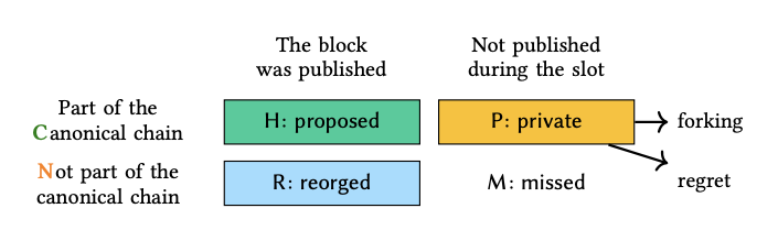
Block statuses are denoted as indicating that the block in the th slot in epoch was proposed, reorged, missed, or built privately, respectively. Reorged and missed blocks do not contribute to the generation of since they are not part of the canonical chain.
2.2.2 Self Mixing Strategy
The adversary can selectively propose or miss blocks to manipulate . Assume that is assigned with consecutive tail blocks, formally of epoch , then can choose arbitrarily between by missing or proposing each tail block. Thus, it is trivial that for , as can compute corresponding to .
The manipulative power for is the following decision tree
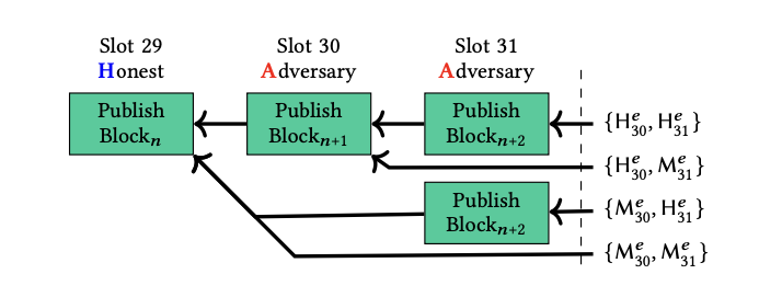
e.g : The adversary chooses option if the calculated eventually leads to the highest number of blocks. In this case, sacrificing Slot 30 and 31 is worthwhile, as it results in a significantly higher number of blocks in epoch .
2.2.3 Forking Strategies
To achieve the goal of maximizing trailing blocks at this critical juncture, the adversary leverages the forking nature of the consensus protocol by introducing a private chain. By strategically applying the Longest-Chain rule to their advantage, the adversary ensures that the last honest trailing blocks are excluded at this pivotal moment. With this added dimension, gaining access to possible combinations of slot leader distributions becomes equivalent to , where and represent the number of adversarial and honest blocks, respectively, within this specific interval of the protocol :
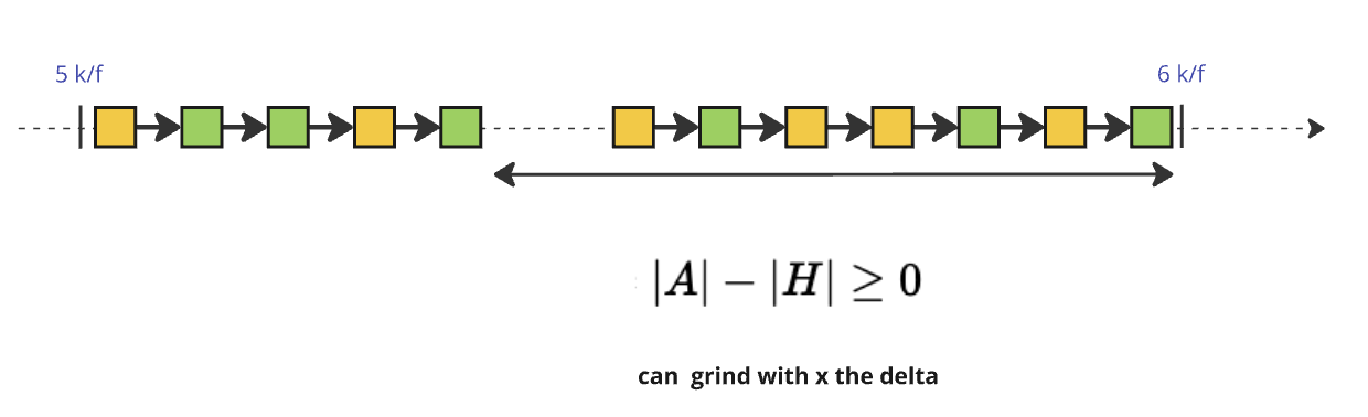
The adversary can choose between two forking strategies depending on when they act:
-
Preemptive Forking (Ex-Ante Reorging): The adversary forks before the randomness update, ensuring that only adversarial VRF contributions are included while honest ones are discarded. This allows them to manipulate before it is finalized, biasing leader selection for the next epoch.
-
Reactive Forking (Ex-Post Reorging): Instead of acting in advance, the adversary waits until all honest VRF contributions are revealed before deciding whether to fork. If the observed is unfavorable, they publish an alternative chain, replacing the honest blocks and modifying the randomness post-facto.
Both strategies undermine fairness in leader election, with Preemptive Forking favoring proactive randomness manipulation and Reactive Forking enabling selective, informed chain reorganizations.
3. The Cost of Grinding: Adversarial Effort and Feasibility
3.1 Definitions
3.1.1 Alpha-Heavy and Heaviness
We define the heaviness of an interval as the percentage of blocks an adversary controls. Let be the number of adversarial blocks and similarly the number of honest blocks in the an interval of blocks. The heaviness of an interval of size is thus the ratio . Heaviness thus vary between 0, where the interval only comprises honest blocks, and 1, where the adversary control them all.
We say that the interval is -heavy if . We furthermore say that the adversary dominates the interval if . We shall look from now on to the longest suffix the adversary dominates at the critical juncture, hence the longest interval where .
3.1.2 Grinding Power g
An -heavy suffix must be present at the critical juncture for a grinding attack to be considered. The heavier , for a fixed , the greater the adversary’s grinding power.
The grinding power of an adversary is the number of distinct values that can choose from when determining for the epoch nonce . This quantifies the adversary's ability to manipulate randomness by selectively withholding, recomputing, or biasing values.
Let be the number of possible grinding attempts in an interval of size when controlling blocks. We have,
The grinding power for a given interval of size is the sum of when the adversary dominates the interval, that is the adverary controls a majority of the blocks.
Similarly, we define the grinding depth, , as the logarithm of the grinding power: , and bound it by . It determines the entropy reduction caused by an adversary's nonce manipulation, directly impacting the protocol's resistance to randomness biasing, that is the number of bits of randomness an adversary can manipulate (we upper bound to 256 as the random nonce is 256-bit long).
In a simplified model where the multi-slot leader feature is not considered, the probability an adversary with stake controls out of blocks is:
where:
- represents the number of ways to select blocks out of .
- is the percentage of stake controlled by the adversary.
We can now define the expected grinding power :
In Cardano mainnet, the nonce size used in the randomness beacon is 256 bits, meaning the theoretical maximum grinding power is . However, practical grinding power is typically limited by computational constraints and stake distribution dynamics.
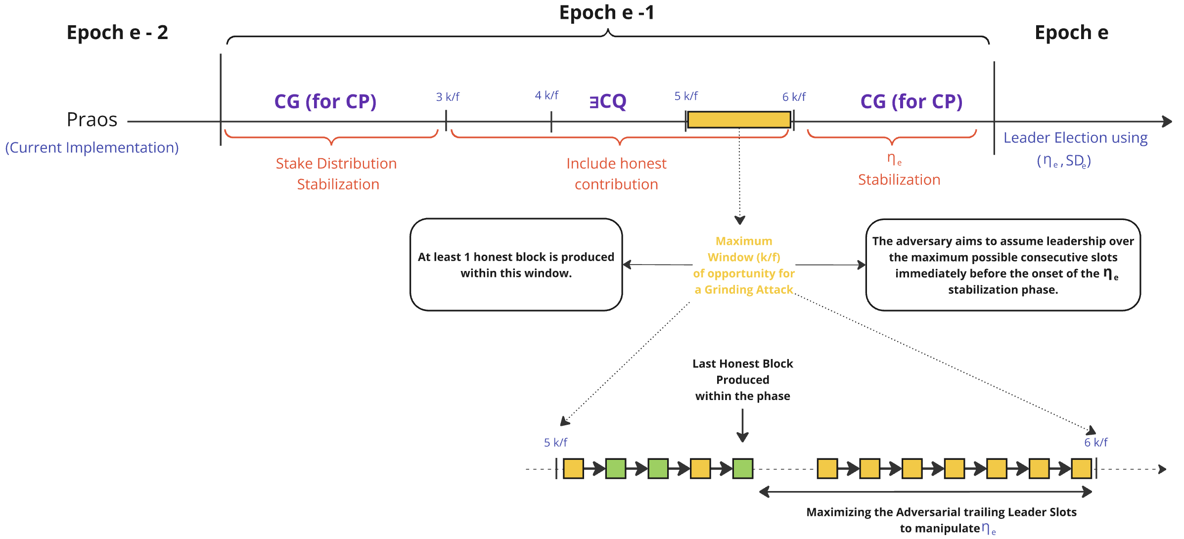
3.1.3 Grinding Windows
3.1.3.1 Opportunity Windows wO
The grinding opportunity window is the time interval at the end of Phase 2 during which an adversary, dominating a suffix of size , can compute and reveal one of possible nonces before the honest chain outpaces their chosen chain.
The end of Phase 2 happens after slots, where is sampled from based on the VRF outputs of blocks up to that point (see Section 1.3.5). Given the protocol parameters and , we have .
Assuming the adversary controls the slots (between slot numbered and ), they can manipulate VRF outputs to generate up to possible nonces by selectively revealing or withholding each output. After , a chain with their chosen nonce — ranging in length from (revealing no blocks, withholding all) to (revealing all) — is set. As such, the grinding oppotunity window is bounded by :
N.B. Contrary to the grinding power that is upper-bounded by , the grinding window is bounded by of Chain Prefix (CP) property.
- Parameters:
- : Active slot coefficient (e.g., ), the fraction of slots with a leader.
- Slot duration = 1 second.
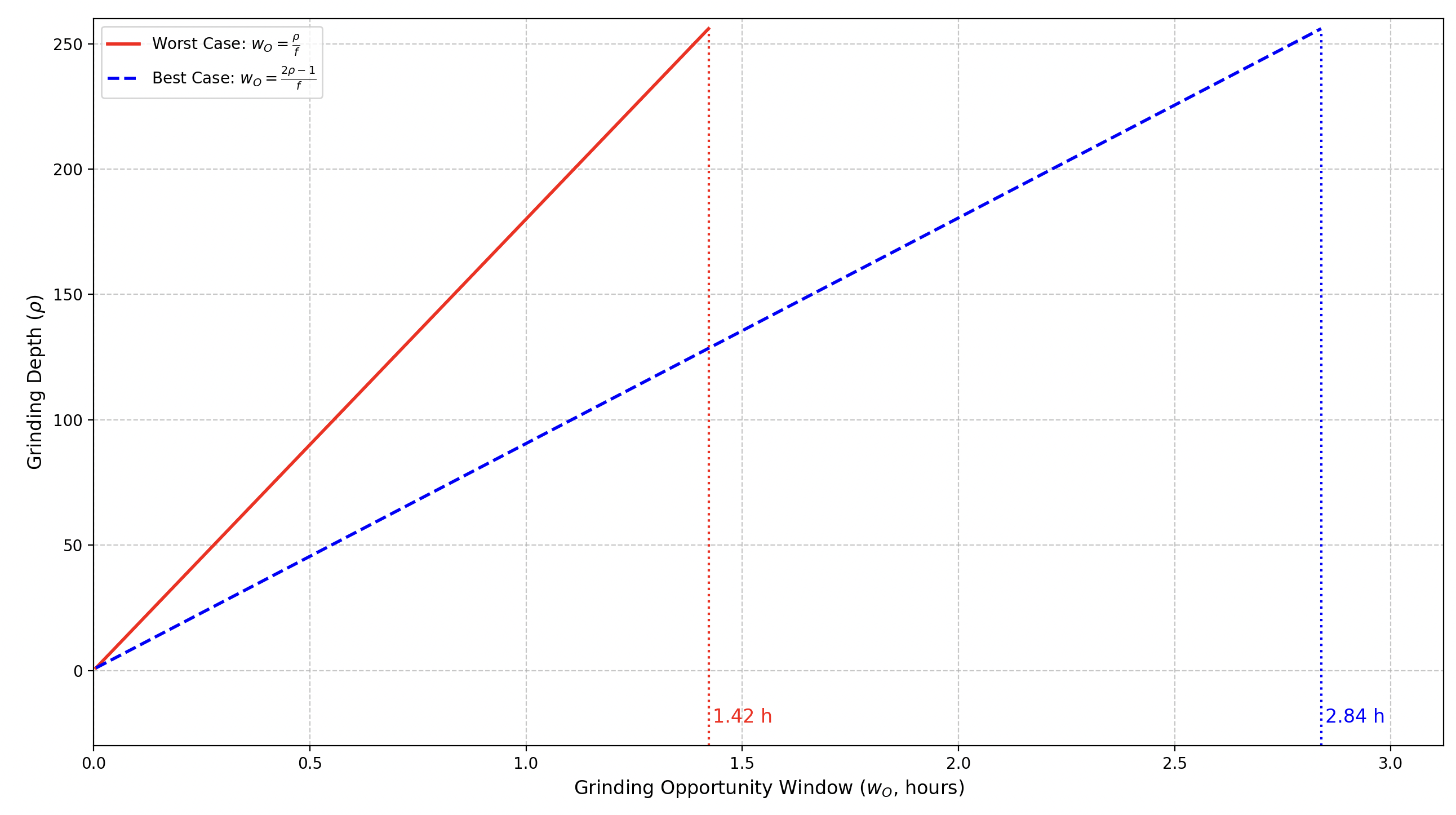
✏️ Note: The code to generate this graph is available at ➡️ this link.
Let's consider the worst case where the adversary controls all trailing slots ():
-
:
- seconds (~5.3 minutes).
- Starts at , ends at (adjusted for reveal timing).
-
:
- seconds (~10.7 minutes).
- Starts at , ends at .
-
:
- seconds (~85.3 minutes).
- Starts at , ends at .
This sizing ensures the adversary has time to act before honest chain growth threatens even a length-1 chain, providing a practical and conservative bound for grinding feasibility.
We can moreover defined opportunity window with respect to the adversarial stake, . The expected opportunity window tends to,
- Parameters:
- : Active slot coefficient (e.g., ), the fraction of slots with a leader.
- is the percentage of stake controlled by the adversary.
- Slot duration = 1 second.
| (%) | 0.5 | 1 | 2 | 5 | 10 | 20 | 25 | 30 | 33 | 40 | 45 | 49 |
|---|---|---|---|---|---|---|---|---|---|---|---|---|
| (s) | 2.02E-01 | 4.08E-01 | 8.33E-01 | 2.22E00 | 5.00E00 | 13.33E00 | 2.00E01 | 3.00E01 | 3.88E01 | 8.00E01 | 1.80E02 | 9.79E02 |
📌📌 More Details on the expectation's computation – Expand to view the content.
To compute the expectation of the opportunity window, we need to find the earliest slot starting from the end of Phase 2, such that the adversary controls a majority of slots in that interval (and before the chain has been set, that is before slots).
More particularly, if we define each slot as a Benoulli random variable such that the slot is takes for value 1 — is owned by the adversary — with probability , we want to compute the expectation of the earliest position such that .
We can make the problem symmetric by defining . In that case, wth probability and with probability . We can rewrite the inequality then as,
By re-indexing, with and , we have, .
We can see this sum over as finding the length of a Gambler's ruin problem with initial stake 0 and sole end condition that the stake becomes negative. As such, we have, (we remove one as ruin is defined as the first time the stake equals ).
The position then becomes and the opportunity window is the duration of the interval from position to the end of the interval of size , hence .
3.1.3.2 Target Window wT
Once the adversary obtains a potential candidate nonce () for epoch , they can compute their private slot leader distribution for the entire epoch, spanning:
We define the grinding target window as the slot interval an adversary targets based on their attack strategy, where .
3.1.3 Grinding Attempt
A grinding attempt is a single evaluation of a possible nonce by the adversary within the grinding target window .
Each attempt follows three key steps:
- Computing a candidate nonce by selectively revealing or withholding VRF outputs.
- Simulating the resulting slot leader distribution over the target window .
- Evaluating the strategic benefit of choosing this nonce for their attack objectives.
The number of grinding attempts an adversary can make is constrained by their grinding power , and is upper-bounded by:
where the adversary dominates the suffix of size at the critical juncture and represents the number of blocks they control in that interval.
3.2 Entry Ticket: Acquiring Stake to Play the Lottery
Before an adversary can execute a grinding attack, they must first acquire enough stake, akin to buying an entry ticket to participate in a lottery.
In this case, the lottery is the leader election process, where the probability of winning a slot—and thus influencing the nonce—is directly proportional to the stake held.
Just like in a lottery, the more tickets an adversary buys (stake accumulated), the greater their chances of winning.
By securing a significant share of stake, they increase the likelihood of being selected as a slot leader in key trailing positions, providing the foundation needed to execute a grinding attack.
Thus, the first cost of a grinding attack is not computational but economic —the price of acquiring enough stake to play the lottery.
To estimate the cost of these entry tickets, we address the following question:
How many blocks can an adversary control on average with a given adversarial stake, ensuring a reasonable probability—such as at least one successful grinding opportunity within 10 years of continuous epoch-by-epoch execution in Cardano, where each epoch lasts 5 days?
Specifically, for a given adversarial stake, we seek the maximum for which the probability of obtaining a dominating -heavy suffix is at least once over 10 years, meaning at least one occurrence within 3,650 epochs.
N.B.: A 10-year period spans two full technological innovation cycles, significantly increasing the likelihood of disruptive advancements in cryptographic research, computing power, or consensus protocols. This timeframe provides a long enough horizon for:
- Assessing long-term adversarial feasibility and whether stake-based grinding remains viable at scale.
- Observing historical adversarial behaviors, particularly in decentralized networks with shifting governance dynamics.
- Giving the Cardano community sufficient time to introduce fundamental protocol-level improvements to Ouroboros that could completely mitigate or transform this issue.
The Data
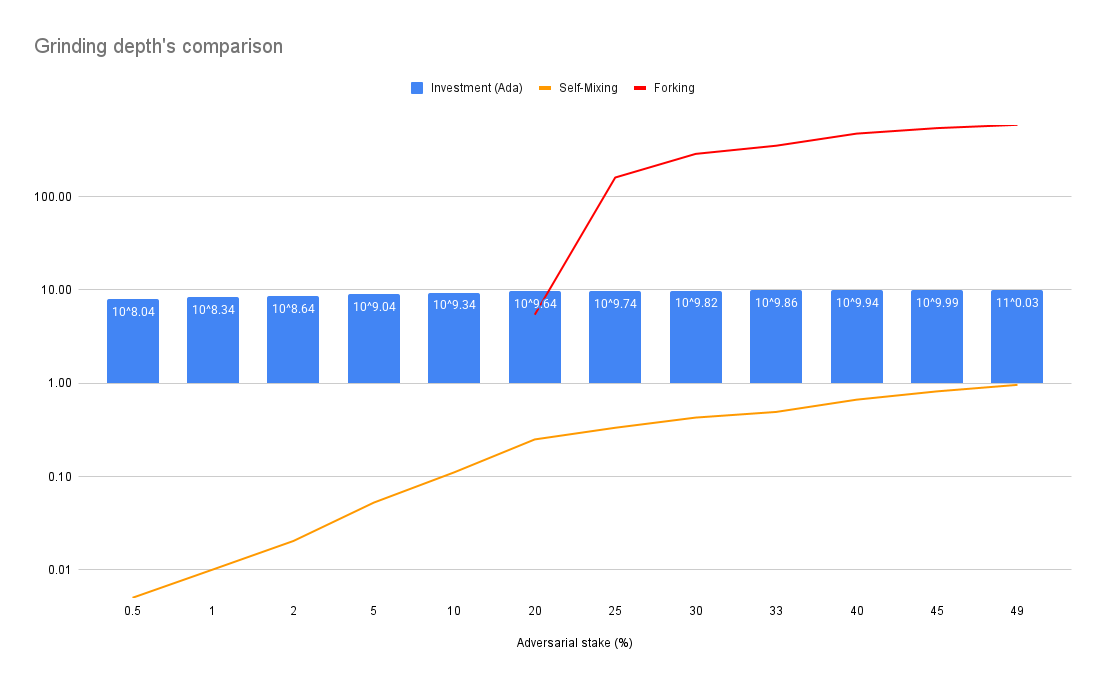
We are computing here the expected number of grinding attempts for both the self-mixing and forking strategies.
Self-Mixing
We present here the average number of years required for an adversary with a stake of to control N blocks. We chose to emphasize frequencies below 10 years, as it is reasonable to assume the protocol will have evolved after such a period.
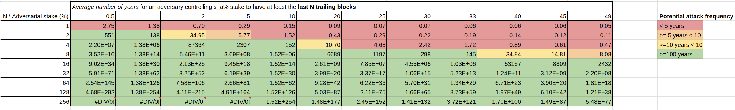
(*) We make the simplification to consider the 21,600 blocks directly, that is: there is only 21,600 slots and to each to slot is exactly assigned one slot leader.
📌📌 More Details on Probabilities Here – Expand to view the content.
We display here the probabilities of an adversary with a stake of controlling N blocks:
| (%) | 0.5 | 1 | 2 | 5 | 10 | 20 | 25 | 30 | 33 | 40 | 45 | 49 |
|---|---|---|---|---|---|---|---|---|---|---|---|---|
| 5.00E-03 | 1.00E-02 | 2.00E-02 | 5.00E-02 | 1.00E-01 | 2.00E-01 | 2.50E-01 | 3.00E-01 | 3.30E-01 | 4.00E-01 | 4.50E-01 | 4.90E-01 | |
| 2.50E-05 | 1.00E-04 | 4.00E-04 | 2.50E-03 | 1.00E-02 | 4.00E-02 | 6.25E-02 | 9.00E-02 | 1.09E-01 | 1.60E-01 | 2.03E-01 | 2.40E-01 | |
| 6.25E-10 | 1.00E-08 | 1.60E-07 | 6.25E-06 | 1.00E-04 | 1.60E-03 | 3.91E-03 | 8.10E-03 | 1.19E-02 | 2.56E-02 | 4.10E-02 | 5.76E-02 | |
| 3.91E-19 | 1.00E-16 | 2.56E-14 | 3.91E-11 | 1.00E-08 | 2.56E-06 | 1.53E-05 | 6.56E-05 | 1.41E-04 | 6.55E-04 | 1.68E-03 | 3.32E-03 | |
| 1.53E-37 | 1.00E-32 | 6.55E-28 | 1.53E-21 | 1.00E-16 | 6.55E-12 | 2.33E-10 | 4.30E-09 | 1.98E-08 | 4.29E-07 | 2.83E-06 | 1.10E-05 | |
| 2.33E-74 | 1.00E-64 | 4.29E-55 | 2.33E-42 | 1.00E-32 | 4.29E-23 | 5.42E-20 | 1.85E-17 | 3.91E-16 | 1.84E-13 | 7.99E-12 | 1.22E-10 | |
| 5.42E-148 | 1.00E-128 | 1.84E-109 | 5.42E-84 | 1.00E-64 | 1.84E-45 | 2.94E-39 | 3.43E-34 | 1.53E-31 | 3.40E-26 | 6.39E-23 | 1.49E-20 | |
| 2.94E-295 | 1.00E-256 | 3.40E-218 | 2.94E-167 | 1.00E-128 | 3.40E-90 | 8.64E-78 | 1.18E-67 | 2.34E-62 | 1.16E-51 | 4.09E-45 | 2.21E-40 | |
| 0.00E+00 | 0.00E+00 | 0.00E+00 | 0.00E+00 | 1.00E-256 | 1.16E-179 | 7.46E-155 | 1.39E-134 | 5.49E-124 | 1.34E-102 | 1.67E-89 | 4.90E-80 |
We present the expected number (i.e., moment) of grinding attempts during self-mixing, which refers to trailing blocks within an epoch.
| (%) | 0.5 | 1 | 2 | 5 | 10 | 20 | 25 | 30 | 33 | 40 | 45 | 49 |
|---|---|---|---|---|---|---|---|---|---|---|---|---|
| 0.005 | 0.010 | 0.020 | 0.053 | 0.111 | 0.250 | 0.333 | 0.429 | 0.493 | 0.667 | 0.818 | 0.961 |
We conclude that the self-mixing attack is neither highly probable nor particularly critical.
Forking
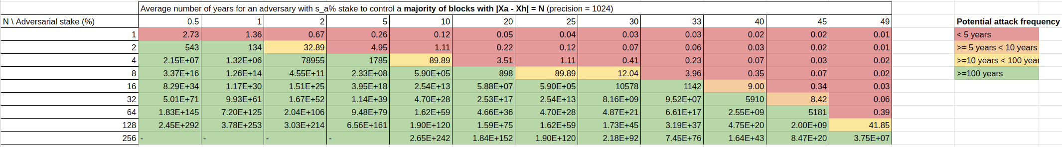
We extend here the self-mixing strategy with forking and show how this renders the attack viable.
We first introduce the formula for the probability for an adversary having stake of having an advantage of blocks, that is an adversary controlling a majority of blocks, in any given interval smaller than blocks where is from the -CQ property.
As the formula is not computationally friendly, instead of showing numbers for an interval of size , we look at a smaller interval of size , to give us a lower-bound on these numbers. We now display a lower bound on the probabilities of having an advantage of blocks, and an upper-bound on the frequency of a corresponding grinding attack per year.
📌📌 More Details on Probabilities Here – Expand to view the content.
We display here the probabilities of an adversary with a stake of controlling a majority of blocks such that :
| (%) | 0.5 | 1 | 2 | 5 | 10 | 20 | 25 | 30 | 33 | 40 | 45 | 49 |
|---|---|---|---|---|---|---|---|---|---|---|---|---|
| 5.00E-03 | 1.00E-02 | 2.00E-02 | 5.00E-02 | 1.00E-01 | 2.00E-01 | 2.50E-01 | 3.00E-01 | 3.30E-01 | 4.00E-01 | 4.50E-01 | 4.90E-01 | |
| 2.50E-05 | 1.00E-04 | 4.00E-04 | 2.50E-03 | 1.00E-02 | 4.00E-02 | 6.25E-02 | 9.00E-02 | 1.09E-01 | 1.60E-01 | 2.03E-01 | 2.40E-01 | |
| 6.25E-10 | 1.00E-08 | 1.60E-07 | 6.25E-06 | 1.00E-04 | 1.60E-03 | 3.91E-03 | 8.10E-03 | 1.19E-02 | 2.56E-02 | 4.10E-02 | 5.76E-02 | |
| 3.91E-19 | 1.00E-16 | 2.56E-14 | 3.91E-11 | 1.00E-08 | 2.56E-06 | 1.53E-05 | 6.56E-05 | 1.41E-04 | 6.55E-04 | 1.68E-03 | 3.32E-03 | |
| 1.53E-37 | 1.00E-32 | 6.55E-28 | 1.53E-21 | 1.00E-16 | 6.55E-12 | 2.33E-10 | 4.30E-09 | 1.98E-08 | 4.29E-07 | 2.83E-06 | 1.10E-05 | |
| 2.33E-74 | 1.00E-64 | 4.29E-55 | 2.33E-42 | 1.00E-32 | 4.29E-23 | 5.42E-20 | 1.85E-17 | 3.91E-16 | 1.84E-13 | 7.99E-12 | 1.22E-10 | |
| 5.42E-148 | 1.00E-128 | 1.84E-109 | 5.42E-84 | 1.00E-64 | 1.84E-45 | 2.94E-39 | 3.43E-34 | 1.53E-31 | 3.40E-26 | 6.39E-23 | 1.49E-20 | |
| 2.94E-295 | 1.00E-256 | 3.40E-218 | 2.94E-167 | 1.00E-128 | 3.40E-90 | 8.64E-78 | 1.18E-67 | 2.34E-62 | 1.16E-51 | 4.09E-45 | 2.21E-40 | |
| 0.00E+00 | 0.00E+00 | 0.00E+00 | 0.00E+00 | 1.00E-256 | 1.16E-179 | 7.46E-155 | 1.39E-134 | 5.49E-124 | 1.34E-102 | 1.67E-89 | 4.90E-80 |
We now tabulatethe grinding power's expectation when looking at different precision . While the expectation converges quickly for small stake, smaller than 20%, we can note it significicantly rises afterwards.
| 0.5% | 1.0% | 2.0% | 5.0% | 10.0% | 20.0% | 25.0% | 30.0% | 33.0% | 40.0% | 45.0% | 49.0% | |
|---|---|---|---|---|---|---|---|---|---|---|---|---|
| 16 | 0.0203 | 0.0414 | 0.0857 | 0.242 | 0.636 | 3.49 | 8.86 | 22 | 36.8 | 108 | 209 | 334 |
| 32 | 0.0203 | 0.0414 | 0.0857 | 0.242 | 0.637 | 5.71 | 43.4 | 384 | 1,290 | 15,100 | 65,700 | 185,000 |
| 64 | 0.0203 | 0.0414 | 0.0857 | 0.242 | 0.637 | 8.93 | 1010 | 145,000 | 2.01e+06 | 3.56e+08 | 7.36e+09 | 6.06e+10 |
| 128 | 0.0203 | 0.0414 | 0.0857 | 0.242 | 0.637 | 13.6 | 786,000 | 2.92e+10 | 6.59e+12 | 2.44e+17 | 1.05e+20 | 6.87e+21 |
| 256 | 0.0203 | 0.0414 | 0.0857 | 0.242 | 0.637 | 20.2 | 6.98e+11 | 1.64e+21 | 9.6e+25 | 1.45e+35 | 2.48e+40 | 9.29e+43 |
| 512 | 0.0203 | 0.0414 | 0.0857 | 0.242 | 0.637 | 29.6 | 7.87e+23 | 7.19e+42 | 2.8e+52 | 6.59e+70 | 1.64e+81 | 1.79e+88 |
| 1024 | 0.0203 | 0.0414 | 0.0857 | 0.242 | 0.637 | 43 | 1.43e+48 | 1.94e+86 | 3.32e+105 | 1.84e+142 | 8.81e+162 | 7.03e+176 |
We can approximate the expected grinding power as an exponential function of the precision, i.e. . Looking at the exponential's based, can tell us precisely when the grinding power becomes rises exponentially, that is when the exponentiaition starts growing instead of decaying. The following graph indeed confirms that 20% is the threshold.
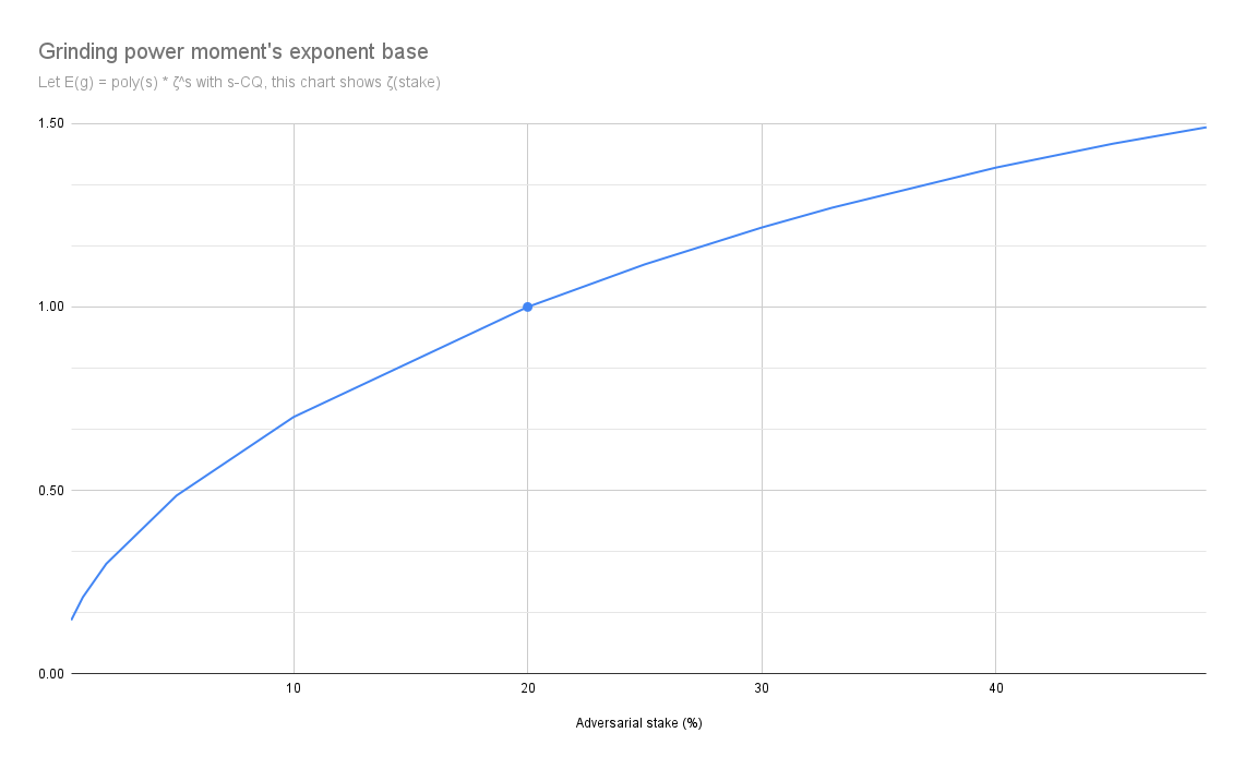
The details of the calculations underlying this table can be found in the following Google Spreadsheet: Details of Calculations.
For example, with 5% adversarial stake, it would take about 1800 years in average for an adversary to obtain an advantage of of exactly 4 blocks at the critical juncture.
The Results
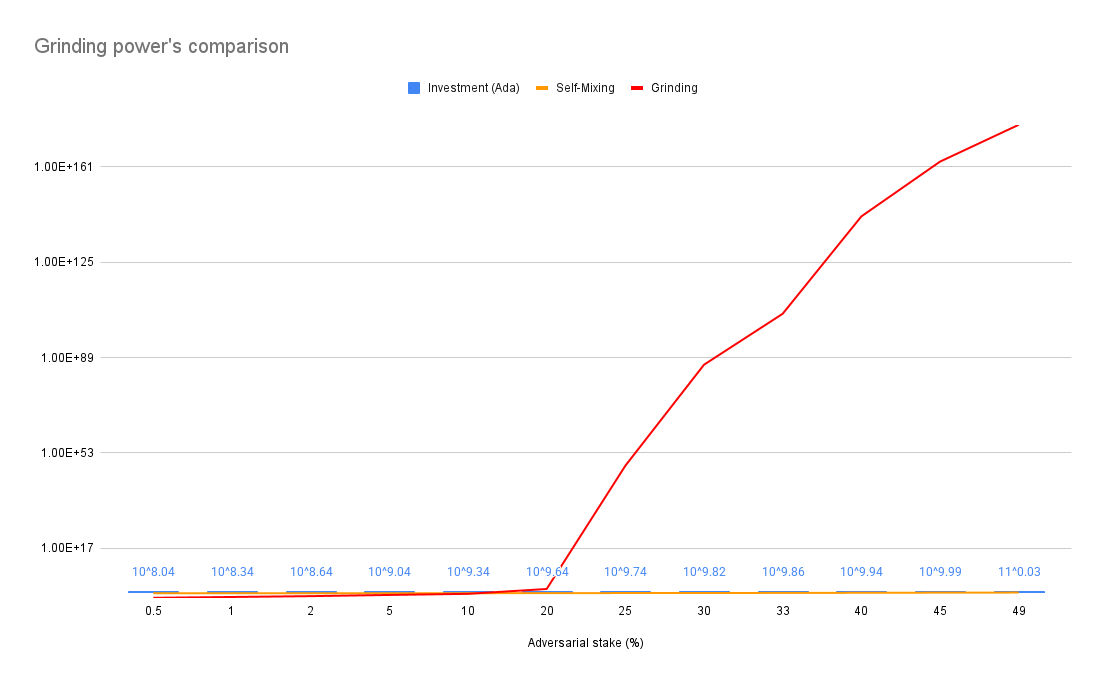
N.B : This analysis does not account for recursion in addition to the forking and self-mixing strategy, so the curve should actually be even steeper than in the graph above.
This investment is non-trivial and serves as an implicit deterrent to attacks, as the adversary must weigh the risks of financial exposure against potential gains. While stake acquisition might appear as a sunk cost, it can, in some cases, be viewed as an active investment in the blockchain ecosystem. For instance, an adversary with a large stake may not only attempt manipulation but could also seek to benefit from staking rewards, governance influence, or other economic incentives, adding an additional layer of strategic decision-making.
Results suggests that crossing the 20% stake threshold dramatically increases an adversary’s probability of influencing leader elections. With such control, their ability to manipulate leader election outcomes becomes exponentially and primarily constrained by computational feasibility rather than probabilistic limitations.
As of March 1, 2025, acquiring a 20% stake in Cardano would require an investment exceeding 4.36 billion ADA, a substantial sum that introduces a fundamental game-theoretic disincentive:
- A successful attack could undermine the blockchain’s integrity, leading to loss of trust and stake devaluation.
- If the attack is detected, reputational damage, delegator withdrawals, or protocol-level countermeasures could make the adversary's stake significantly less valuable.
This reinforces transparency as a natural deterrent: publicly observable grinding attempts expose adversarial stake pool operators (SPOs) to severe economic and social consequences.
3.3 Cost of a Grinding Attempt
As previously explained, each attempt consists of three key steps:
- Computing a candidate nonce by selectively revealing or withholding VRF outputs.
- Simulating the resulting slot leader distribution over the target window .
- Evaluating the strategic benefit of choosing this nonce for adversarial objectives.
Let's analyze each of these steps.
3.3.1 Nonce Generation
We will denote this step as moving forward.
Nonce generation consists of:
- VRF Evaluation: Computes a candidate nonce.
- Operation: Concatenation + BLAKE2b-256 hashing.
Since the VRF outputs can be precomputed, we can discard them from the computational cost of a grinding attack. As for the computational cost, as the hash functions are protected against extension attacks, we have to consider the average cost of hashing of all nonces when considering a fixed grinding depth .
We make the assumption that hashing inputs takes as much time as hashing times two inputs, that is that the finalization step of a hashing function is not significant. We also look at the worst case scenario, for simplification, and assume that .
N.B. We may drop the superscript for readibility.
N.B. This represents the average time to compute a nonce. While each nonce can be computed in parallel, we cannot easily parallelize the generation of one nonce as the computation is sequential.
3.3.2 Slot Leader Distribution Evaluation
We will denote this step as moving forward.
After generating a candidate nonce, the adversary must evaluate its impact on slot leader election over an target window :
- Computing VRF outputs for all slots in of interest.
- Evaluating the eligibilty of these values to know when the adversary is the slot leader.
Since leader eligibility is unknown in advance, the adversary must verify all slots in .
Define:
- → target window size (seconds).
- → VRF evaluation time.
- → Slot eligilibity check.
Each slot requires one VRF verification, leading to:
This represents the total time of the leader distribution evaluation. Once a nonce is computed, we can generate and check the eligibility of the VRF outputs in parallel.
3.3.3 Strategic Benefit Evaluation
We denote this step as moving forward.
After simulating the leader election distribution, the adversary must determine whether the selected nonce provides a strategic advantage by:
- Assessing block production gains relative to honest stake.
- Estimating adversarial control over leader election.
- Comparing multiple nonces to select the most effective one.
Nature of the Computational Workload
Unlike previous steps, this phase does not perform a single deterministic computation but operates as an evaluation loop over a dataset of adversarial leader election scenarios. The attacker’s dataset includes:
- Nonce-to-leader mappings → which nonces yield better leadership control.
- Stake distributions → impact of adversarial stake on slot control.
- Slot timing predictions → evaluating when it's best to control a block.
- Secondary constraints → network conditions, latency factors, or additional attack-specific considerations.
Since this "database" of possible leader elections depends on adversarial strategies, the cost is too diverse to define precisely. While the exact cost varies, this step is compulsory and must be factored into the total grinding time.
3.3.4 Total Estimated Time per Grinding Attempt
The total grinding time is the sum of:
- Nonce Generation () → VRF evaluation + hashing.
- Slot Leader Simulation () → Eligibility checks over .
- Strategic Evaluation () → Nonce selection analysis.
Total Grinding Time Formula
Expanding each term:
- Nonce Generation: :
- Slot Leader Verification :
- Strategic Evaluation : (attack-dependent term)
Final expression:
Where:
- is the VRF evaluation time.
- is the eligibility checktime.
- is the time for the hashing operation.
- is the target window size (seconds).
- is the grinding power.
- is the nonce selection and evaluation time, which is attack-specific.
3.4 Cost of a Grinding Attack
3.4.1 Formula
A grinding attack consists of multiple grinding attempts executed within the grinding opportunity window . Since each grinding attempt takes time to compute, the feasibility of the attack depends on whether the total computation can be completed within this window.
We define the total attack time as:
where:
- = grinding depth (bits of entropy the adversary can manipulate),
- = time required for one grinding attempt,
- = number of CPUs available for parallel execution.
For the attack to be feasible, this total time must fit within the grinding opportunity window :
which leads to the lower bound on computational power () :
Expanding
From Section 3.3, the per-attempt grinding time is:
Substituting this into the inequality:
Expanding in Terms of and
From previous sections, the grinding opportunity window is:
Substituting this into our equation:
3.4.2 Estimated Formula Using Mainnet Cardano Parameters
Starting from the final expression at the end of the last section:
Applying Cardano Mainnet Parameters
Using Cardano’s mainnet values:
- seconds (1 microsecond) – Time to evaluate a Verifiable Random Function.
- seconds (0.01 microseconds) – Time for a BLAKE2b-256 hash operation.
- – Active slot coefficient.
- Slot duration = 1 second.
Thus, the expression becomes:
where each step contributes as follows,
- Nonce Generation: :
- Slot Leader Verification :
- Strategic Evaluation :
Final Expression
The estimated number of CPUs required is:
- : The number of blocks controlled by the adversary.
- : The target window (in seconds), ranging from short (e.g., 3600 s) to a full epoch (e.g., 432,000 s), as defined in Section 3.5 - Scenarios.
- : The strategic evaluation time (in seconds), varying from 0 to 1, as explored in Section 3.5 - Scenarios.
This expression transitions the theoretical cost model into a practical estimate, with specific values for and evaluated in Section 3.5 - Scenarios to assess feasibility across different attack strategies.
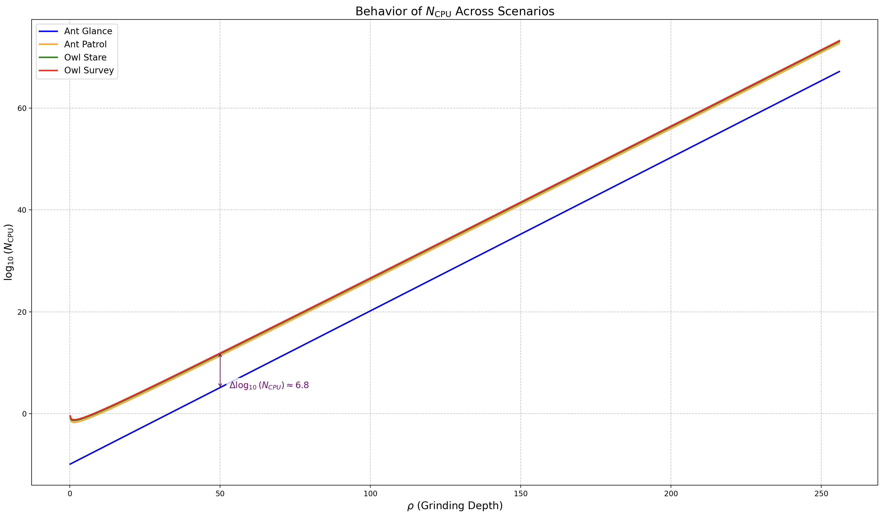
3.5 Scenarios
Following the computational model from Section 3.4.2 - Estimated Formula Using Mainnet Cardano Parameters, we explore four scenarios to observe how randomness manipulation behaves across varying grinding depths . These scenarios are framed with an animal-inspired metaphor reflecting evaluation complexity () and observation scope (), providing a basis for graphical analysis to be developed later.
| Scenario | (Complexity) | (Scope) | Description |
|---|---|---|---|
| Ant Glance | 0 (Low) | 0s | An ant quickly glancing at a small spot, representing simple evaluation (low ) with basic effort and a narrow observation scope (minimal ). |
| Ant Patrol | 0s (Low) | 5d (432,000 s) | An ant patrolling a wide area over time with simple instincts, representing simple evaluation (low ) with basic effort and a broad observation scope (large ). |
| Owl Stare | 1s (High) | 0s | An owl staring intently at a small area with keen focus, representing complex evaluation (high ) with advanced effort and a narrow observation scope (minimal ). |
| Owl Survey | 1s (High) | 5d (432,000 s) | An owl surveying a wide range with strategic awareness, representing complex evaluation (high ) with advanced effort and a broad observation scope (large ). |
The formulas are derived by substituting the respective and values from each scenario into the base expression :
| Scenario | Formula |
|---|---|
| Ant Glance | |
| Ant Patrol | |
| Owl Stare | |
| Owl Survey |
✏️ Note: The code to generate this graph is available at ➡️ this link.
The maximal delta (Owl Survey minus Ant Glance) is now approximately , reflecting a dramatic difference in computational requirements between the simplest and most complex scenarios. This illustrates that and together form a pre-exponential amplification of up to CPUs, which is then further scaled by the exponential factor . The yellow line (Ant Patrol) sits between the blue (Ant Glance) and red (Owl Survey) lines, with a delta of approximately from Ant Glance, confirming that its high s causes a ~120x CPU increase relative to Ant Glance, despite both having .
The green line (Owl Stare), lies below the red line (Owl Survey), with a delta of approximately 0.16 in .
At :
- Ant Glance (, ): ,
- Ant Patrol (, ): ,
- Owl Stare (, ): ,
- Owl Survey (, ): ,
3.6 Grinding Power Computational Feasibility
Building on the analysis in previous Section 3.5, we assessed the feasibility of grinding attacks by examining the computational resources () required across different grinding depths (). The scenarios (Ant Glance, Ant Patrol, Owl Stare, Owl Survey) show a consistent , meaning the most demanding scenario (Owl Survey) requires times more CPUs than the least demanding (Ant Glance).
To help readers understand the practicality of these attacks, we define feasibility thresholds based on economic and computational viability, as shown in the table below:
| Feasibility Category | Cost Range (USD) | Description |
|---|---|---|
| Trivial | < $10,000 | Representing an amount easily affordable by an individual with basic computing resources, such as a personal computer. |
| Feasible | 1,000,000 | Reflects costs that require a substantial financial commitment, typically beyond the reach of individuals but manageable for well-funded entities, such as tech startups, research groups, or organized crime syndicates, assuming access to mid-tier cloud computing resources or a dedicated server farm, necessitating a strategic investment that signals a serious intent to exploit the network. |
| Possible | 1,000,000,000 | Reflects costs that demand resources on the scale of large corporations, government agencies, or nation-states, implying the use of extensive computational infrastructure (e.g., data centers) and significant capital, suggesting an attack that requires coordinated effort and advanced planning, potentially involving millions of CPU hours or specialized hardware. |
| Borderline Infeasible | 1,000,000,000,000 | Indicates costs that approach the upper bounds of what global economies can sustain for a single project, requiring resources comparable to those of major international organizations or coalitions, pushing the limits of current computational and financial capabilities, and suggesting that such an endeavor would strain even well-resourced entities, making it highly improbable without global-scale coordination. |
| Infeasible | > $1,000,000,000,000 | Denotes costs exceeding 1 trillion usd, deemed infeasible because they surpass the total economic output or computational capacity available globally (e.g., estimated at CPUs or `\sim \100`$ trillion GDP as of 2025), implying an attack that is theoretically possible only with resources beyond current technological or economic limits, rendering it practically impossible with present-day infrastructure. |
The cost model uses the formulas from Section 3.5 - Scenarios, computes the number of CPUs needed for the attack, and multiplies by the CPU rental price ( per CPU-hour) and runtime defined by the grinding opportunity window seconds (with ) to estimate the total cost.
Costs are estimated assuming a CPU rental price of per CPU-hour, based on low-end instance pricing from major cloud providers like AWS as of March 11, 2025, where basic instances such as t2.micro cost approximately per CPU-hour AWS EC2 Pricing Page. However, for high-performance tasks, actual costs may range from to per CPU-hour, as seen with AWS c5.large () or Azure Standard_F2s_v2 ().
The table below summarizes the feasibility for Owl Survey (, ), the most resource-intensive scenario, at different values, using the estimate for initial assessment:
| CPUs Required (Log₁₀ Scale) | Estimated Cost (USD) | Feasibility | |
|---|---|---|---|
| 31 | CPUs | 8,394.76 | Trivial for any adversary |
| 37 | CPUs | 539,954 | Feasible with standard resources |
| 47 | CPUs | 553.79 million | Possible with large-scale infrastructure |
| 48 | CPUs | 1.107 billion | Borderline Infeasible, requires massive resources |
| 58 | CPUs | 1.137 trillion | Infeasible, exceeds global computing capacity |
- CPUs Required: Computed for Owl Survey at each , rounded to the nearest order of magnitude for readability (exact values approximated).
- Cost: Assumes per CPU-hour, scaled for the runtime seconds.
- Feasibility: Assessed based on computational and economic viability, considering global computing resources (e.g., CPUs in modern data centers, CPUs globally as of March 11, 2025).
📌 Example Calculation for ρ = 50 (Owl Survey)
Let’s walk through the calculation for the Owl Survey scenario at to demonstrate how the values in the table are derived. The Owl Survey scenario has (high complexity) and (5 days), making it the most resource-intensive scenario.
Step 1: Compute
The formula for in the Owl Survey scenario, as given in Section 3.5 - Scenarios, is:
For , the expression becomes:
In scale:
Step 2: Compute the Estimated Cost in USD
The cost is calculated as
- Cost per CPU-hour: ,
- Runtime: seconds, with :
Step 3: Determine Feasibility
The feasibility thresholds are:
- Trivial: < (),
- Feasible: to ( to 6),
- Possible: to ( to 9),
- Borderline Infeasible: to ( to 12),
- Infeasible: > ().
This scenario is thus Borderline Infeasible, as the cost of falls between and .
✏️ Note: The code to generate this graph is available at ➡️ this link.
The cost difference between the most expensive scenario (Owl Survey) and the cheapest (Ant Glance) is significant, with a consistent , meaning Owl Survey costs approximately times more than Ant Glance, reflecting the substantial impact of and on resource demands.
The table below shows the values where each scenario transitions across feasibility categories:
| Feasibility Category | 🔵 Ant Glance | 🟠 Ant Patrol | 🟢 Owl Stare | 🔴 Owl Survey |
|---|---|---|---|---|
| 🟢 🌱 Trivial for Any Adversary | ||||
| 🟡 💰 Feasible with Standard Resources | ||||
| 🟠 🏭 Large-Scale Infrastructure Required | ||||
| 🔴 🚫 Borderline Infeasible | ||||
| 🔴 🚫 Infeasible |
4. References
-
KRD017 - Ouroboros- A provably secure proof-of-stake blockchain protocol
-
DGKR18 - Ouroboros Praos/ An adaptively-secure, semi-synchronous proof-of-stake blockchain
-
The combinatorics of the longest-chain rule: Linear consistency for proof-of-stake blockchains
-
Efficient Random Beacons with Adaptive Securityfor Ungrindable Blockchains
-
Forking the RANDAO: Manipulating Ethereum's Distributed Randomness Beacon
5. Copyright
This CIP is licensed under Apache-2.0.